Monetary policy implementation and the consolidated government balance sheet
Central banks typically pursue their macroeconomic objectives by changing short-term interest rates to speed or slow economic activity.[1] The desired setting of short-term rates is known as the stance of monetary policy. After selecting a monetary policy stance, the central bank must employ its tools to influence short-term rates to implement that stance.
These tools consist, broadly speaking, of adjustments in the quantities or prices of the central bank’s liabilities (such as reserves that it supplies to commercial banks) or assets (such as government securities that it acquires to back the reserves it issues). Central banks have multiple tools, so they can implement the same policy stance with a variety of methods. Policymakers and practitioners have debated the merits of different approaches.
A core consideration in these debates has been which implementation methods are most efficient and effective for monetary policy purposes.[2] However, central banks in most jurisdictions are governmental or quasi-governmental entities. As such, when central banks adjust their assets and liabilities, they also change the consolidated balance sheet and income statement of the government as a whole.
This essay examines the trade-offs between different monetary policy implementation methods through the lens of the consolidated government balance sheet and income statement. How does monetary policy implementation influence the government’s revenue and expenses, the risks that taxpayers bear and the efficiency with which the government can accomplish society’s goals?
A central insight is that the choice between different monetary policy implementation methods is also a choice between different fiscal policies: Changing the implementation method can change the government’s source or amount of tax revenue without changing the stance of monetary policy. Accordingly, standard ideas from optimal tax theory can shed light on the optimality of various approaches to monetary policy implementation.
To illustrate this point, consider the trade-offs between two monetary policy implementation approaches commonly employed in developed economies in recent decades. In an ample-reserves regime—employed by the Federal Reserve since 2008—the central bank supplies enough reserves to commercial banks to satiate their demand for reserves with money market rates close to the interest rate paid on reserves. In a scarce-reserves regime—employed by the Federal Reserve before 2008—the central bank reduces the supply of reserves to the point where they carry a scarcity premium, and money market interest rates settle above the interest rate on reserves.
The stance of monetary policy in either regime refers to money market rates. Accordingly, holding the stance of policy constant, the scarce-reserves regime features a smaller supply of reserves and a lower interest rate on reserves than the ample-reserves regime. Reserves are a liability of the consolidated government. Thus, the scarce-reserves regime reduces the amount and cost of one type of government debt. So that the consolidated government’s assets and liabilities continue to balance, the consolidated government must then either issue more debt of some other type (such as government securities) or hold fewer assets (for example, the central bank could reduce its holdings of nongovernment assets), relative to the ample-reserves regime. The cost of alternative debt and the returns on alternative assets determine the net implications for taxpayers of the different implementation regimes.
Suppose the government makes up for the reduction in reserves in the scarce-reserves regime by issuing more overnight government securities. To find a buyer, these securities will need to pay the market interest rate, so the reduced quantity of reserves relative to the ample-reserves regime is exactly offset by increased government debt issuance paying the same interest rate as before. However, because the interest rate on the remaining reserves is below the market rate, the total net interest expense recorded on the government’s income statement is lower in the scarce-reserves regime.
This change does not mean the consolidated government can reduce effective taxes, though. The reduction in the government’s net interest expense exactly matches a reduction in commercial banks’ net interest income from holding reserves that now earn a below-market interest rate. Thus, the scarce-reserves regime effectively taxes commercial banks’ reserve holdings. Whether such a tax is optimal for society depends on how banks respond to it and on the other tax instruments available to the government.
The essay proceeds as follows:
- Section 1 constructs a stylized model of the central bank and government balance sheets and income statements. The model employs a simplified environment where there is no duration risk or friction between money markets and where the central bank’s assets consist only of government securities.
- Section 2 shows how the consolidated balance sheet and income statement in this simplified environment change across the ample-reserves and scarce-reserves implementation regimes.
- Section 3 examines the two regimes in the light of optimal tax theory. I argue that, from a fiscal perspective, the scarce-reserves regime is preferable to the ample-reserves regime only if banks’ reserve holdings cause negative externalities, or banking activities are less elastically supplied or demanded than other activities that the government could tax instead.
- Section 4 examines the implications for the consolidated balance sheet and income statement if the central bank supplies more-than-ample reserves.
- Section 5 extends the model by expanding the asset space: The finance ministry can issue long-term securities, and the central bank can hold assets that are not government debt, such as loans to commercial banks. I show that the mix of assets held by the central bank influences the fiscal risks to which taxpayers are exposed. When the central bank holds nongovernment assets, the consolidated government effectively takes on leverage to invest in the private sector.
- Section 6 is the conclusion.
1. The consolidated government balance sheet and income statement
I consider a government consisting of a finance ministry and a central bank. The finance ministry’s liabilities are overnight finance ministry debt D, which may be held by the private sector (DP) or the central bank (DCB). Expected net future tax revenue TF backs these liabilities. The central bank’s liabilities are reserves R, which it backs with finance ministry debt DCB. (For simplicity, I abstract from currency, and I assume for now that all debt is overnight.) Table 1 shows the respective balance sheets of the finance ministry and the central bank.
| Finance ministry—assets | Finance ministry—liabilities |
| TF | DP |
| DCB |
| Central bank—assets | Central bank—liabilities |
| DCB | R |
The consolidated government balance sheet combines the assets and liabilities of the finance ministry and central bank. DCB cancels out in the combined balance sheet because it is a liability of the finance ministry and an asset of the central bank. Table 2 shows the consolidated government balance sheet.
| Consolidated government—assets | Consolidated government—liabilities |
| TF | DP |
| R |
The finance ministry, central bank and consolidated government also have income statements. I assume that the central bank remits its net income to the finance ministry. The finance ministry’s revenue thus consists of taxes T and central bank net income Z, while its expenses are government expenditures G and interest on the debt I.[3]
I assume there are no frictions between different money markets. Accordingly, all overnight money market instruments carry the same interest rate. The central bank’s policy stance is thus represented by the overnight market interest rate on finance ministry debt r. The finance ministry’s interest expense is I = r*(DP + DCB).
The central bank remunerates reserves at interest rate rR, which could differ from the market rate r. The central bank’s expenses consist of interest on reserves and remittances to the finance ministry, while its revenue comes from interest on its finance ministry debt holdings. (I abstract from operational expenses, which for most central banks are minimal relative to the cash flows from assets and liabilities.) Table 3 shows the income statements of the finance ministry and central bank. Table 4 shows the consolidated government income statement, in which interest on debt held by the central bank and central bank remittances to the finance ministry each cancel out.
| Finance ministry—revenue | Finance ministry—expenses |
| T | r*DP |
| Z | r*DCB |
| G |
| Central bank—revenue | Central bank—expenses |
| r*DCB | rR*R |
| Z |
| Consolidated government—revenue | Consolidated government—expenses |
| T | G |
| r*DP | |
| rR*R |
To close the model, it is necessary to describe the behavior of the private sector agents that may hold reserves and finance ministry debt as assets. The private sector consists of banks and nonbanks. Both banks and nonbanks may own finance ministry debt. Banks may also own reserves; nonbanks may also own deposits at banks.
I assume nonbanks’ demand for both finance ministry debt and bank deposits is increasing in the market interest rate r. Nonbanks’ demand for finance ministry debt is DP,NB = FNB(r) where F'NB > 0, and nonbanks’ demand for bank deposits is FB(r) where F'B > 0.
In this simplified environment, I assume commercial banks’ assets consist only of reserves and finance ministry debt, financed solely with deposits: DP,B + R = FB(r). Because the quantity of deposits is increasing in r, banks’ demand for the sum of reserves and finance ministry debt is increasing in r. (Although banks in this simple model do not issue equity, face leverage constraints, borrow from the central bank or lend to the private sector, a more complex model with those features could also generate an upward-sloping demand for reserves plus finance ministry debt.)
Finally, I assume banks’ demand for reserves depends on the relative yields of reserves and finance ministry debt, and that banks choose to hold some reserves for payments or regulatory purposes even when the interest rate on reserves is below market rates. Thus, banks’ demand for reserves is R = H(Δ) where the spread between money market rates and interest on reserves is Δ = r – rR and where H'(Δ) < 0.
Total finance ministry debt held by the private sector is the sum of finance ministry debt held by banks and nonbanks: DP = DP,B + DP,NB. It will be convenient to define the total demand for government liabilities—both finance ministry debt and reserves—as F(r) = FB(r) + FNB(r).[4]
2. Consolidated balance sheet and income statement across policy implementation regimes
This section considers how the consolidated government balance sheet and income statement change across two illustrative policy implementation regimes, one with ample reserves and the other with scarce reserves. In both regimes, the stance of monetary policy is the same: The central bank adjusts its tools so that the market rate on overnight government debt is r.
I assume expected future tax revenue TF does not vary across the regimes. This assumption implies total finance ministry debt D = DP + DCB is likewise constant across regimes.
I further assume the government adjusts current taxes T across regimes to hold its consolidated net income or deficit unchanged: T–G–r*Dp – rR*R = Q where Q is constant.
This regime is similar to that currently employed by the Federal Reserve.
- The central bank supplies a quantity of reserves RA that meets banks’ demand with market rates equal to interest on reserves. Thus, rR=r and RA = H(0).
- The central bank changes the stance of policy by changing the interest rate on reserves rR. Arbitrage keeps the market interest rate the same as the interest rate on reserves.[5]
- Finance ministry debt to the central bank is the quantity needed to back ample reserves: DCB,A = RA.
- Finance ministry debt to the private sector is DP,A = D – DCB,A = D – RA. Banks and nonbanks must together hold this debt, so D = F(r).
- Taxes are TA = Q + G + r*(DP,A + RA) = Q + G + r*F(r).
Tables 5 and 6 show the consolidated government balance sheet and income statement in this regime.
| Consolidated government—assets | Consolidated government—liabilities |
| TF | DP,A = D – RA = F(r) – RA |
| RA |
| Consolidated government—revenue | Consolidated government—expenses |
| TA = Q + G + r*F(r) | G |
| r*DP,A + r*RA = r*F(r) |
This regime is similar to that employed by the Federal Reserve before 2008.
- The central bank sets the interest rate on reserves below the market rate, rR = r – Δ. It supplies a quantity of reserves RS = H(Δ) < RA that meets banks’ demand given this interest rate.
- The central bank changes the policy stance by changing either the supply of reserves RS, so that Δ changes, or rR.[6]
- Finance ministry debt to the central bank is the quantity needed to back scarce reserves: DCB,S = RS.
- Finance ministry debt to the private sector is DP,S = D – DCB,S = D – RS. Banks and nonbanks must together hold this debt, so, as in the ample-reserves regime, D = F(r).
- Taxes are TS = Q + G + r*DP,S + rR*RS = Q + G + r*(D – RS) + rR*RS = TA – Δ*RS.
Tables 7 and 8 show the consolidated government balance sheet and income statement in this regime.
| Consolidated government—assets | Consolidated government—liabilities |
| TF | DP,S = D – RS = F(r) – RS |
| RS |
| Consolidated government—revenue | Consolidated government—expenses |
| TS = TA – Δ*RS | G |
| r*DP,S + rR*RS = r*F(r) – Δ*RS |
Relative to the ample-reserves regime, if the government deficit is held constant, the government collects Δ*RS less in taxes, making up this revenue by paying Δ*RS less in total interest expense. The government achieves this interest savings while maintaining the same total liabilities because banks hold reserves that are remunerated below the market rate. Effectively, banks in this regime pay an implicit tax of Δ*RS that they did not pay in the ample regime.
The consolidated government’s total liabilities are the same in both regimes: D = F(r). However, the composition of liabilities varies across regimes. Chart 1 illustrates this variation. The scarce-reserves regime increases consolidated finance ministry debt to the private sector relative to the ample-reserves regime.
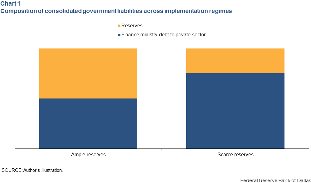
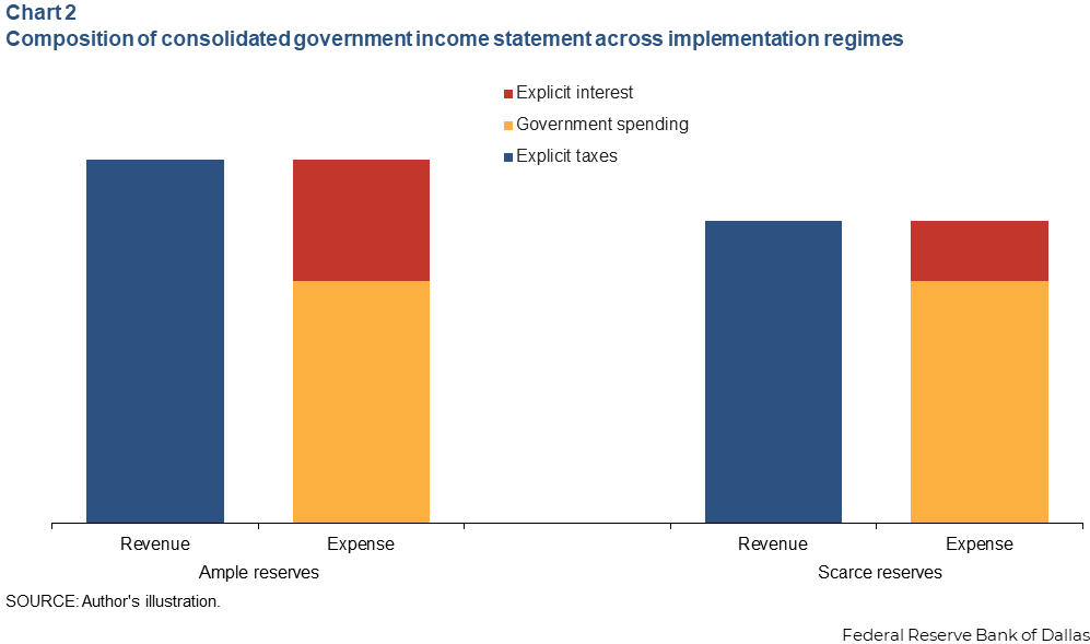
Chart 2 graphically summarizes the variation in the consolidated government income statement across the two policy implementation regimes. The government’s consolidated explicit interest expense—interest on finance ministry debt and reserves—is lower when the central bank supplies scarce reserves than when it supplies ample reserves. Correspondingly, explicit taxes are also lower under scarce reserves.
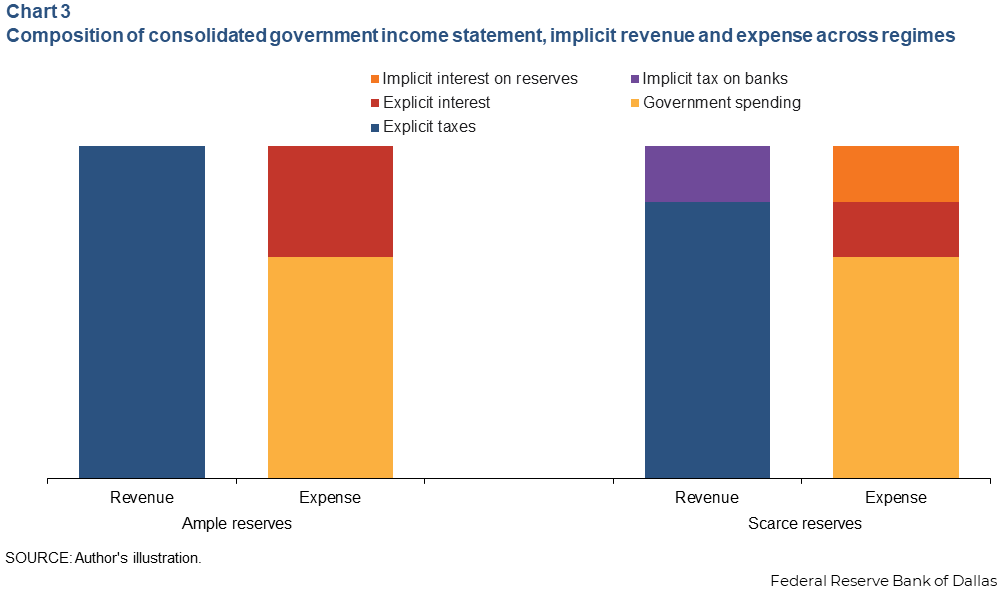
How does the government support the same spending G and the same total consolidated liabilities D with less tax revenue in the scarce-reserves regime? With scarce reserves, the government has additional implicit revenue and expenses that are not visible on the consolidated income statement. Reserves remunerated below market rate carry an implicit interest expense equal to the spread to market rate, but the government does not pay this expense in cash. Rather, the expense is covered by an implicit tax on banks that hold reserves. Chart 3 shows the consolidated government income statement with the inclusion of implicit revenue and expenses. With the inclusion of implicit revenue and expenses, the consolidated government has the same total revenue and expenses under both implementation regimes.
3. Optimal taxation and monetary policy implementation
Taxes influence private behavior. This influence can promote or interfere with achieving desirable outcomes for society, depending on the design of the taxes. Two well-known results from optimal tax theory are:
- Pigouvian taxes and subsidies: The government should tax goods and services that create negative externalities and subsidize those that create positive externalities to offset the externalities.[7]
- Ramsey taxes: After correcting externalities, if the government needs to raise a specified amount of revenue, it should impose heavier taxes on goods and services whose supply and demand are less elastic. Taxing such goods and services produces a smaller supply and demand response and, therefore, distorts the economy less.[8]
Both results are relevant to the choice of monetary policy implementation regime. As discussed, the scarce-reserves regime entails a tax on banks, whose size is proportional to their reserve holdings, and correspondingly lower taxes on the rest of the economy, relative to the ample-reserves regime. Whether such a tax on banks is socially efficient depends on the externalities, if any, associated with banks’ reserve holdings and on the relative elasticities of supply and demand for banking and for other economic activities.
A tax on banks’ reserve holdings would be socially efficient if banks caused negative externalities on other economic agents by holding reserves. In practice, however, banks’ reserve holdings can create positive externalities in at least two ways.
First, the payments system operates more efficiently when banks hold more reserves and do not need to delay outgoing payments until they receive incoming ones.[9]
Second, increased reserve holdings can make a bank more resilient to liquidity shocks. To the extent that a bank’s failure would impose negative externalities on other economic agents, such as by causing a loss to the government’s deposit insurance fund or to other financial institutions, increased reserve holdings benefit society beyond the benefit to the bank itself.
Thus, the Pigouvian argument suggests that, if anything, banks’ reserve holdings ought to be subsidized, rather than taxed as they are in the scarce-reserves regime.
In practice, when banks’ reserve holdings create positive externalities, the government can induce banks to hold more reserves either by subsidizing reserves or by adopting regulations that require or encourage reserve holdings beyond those a bank would choose on its own. The trade-offs between incentivizing behavior through prices or regulation are beyond the scope of this essay.[10] To the extent that regulations already incentivize reserve holdings, additional subsidies would provide less benefit.
Because the ample-reserves regime neither taxes nor subsidizes banks’ use of reserves, the regime satisfies a version of the Friedman rule.[11] This rule, proposed by economist Milton Friedman, observes that it is efficient for the marginal cost of holding money to equal the social marginal cost of supplying money. If the central bank can create money costlessly, the Friedman rule says the marginal cost of holding money should also be set to zero. Friedman considered an environment in which all money was currency, which does not earn interest; thus, the marginal cost of holding money was the nominal market interest rate, and the rule called for setting the nominal interest rate to 0 percent. In an environment where reserves bear interest, the rule instead calls for eliminating the spread between the market overnight interest rate and the interest rate on reserves, i.e., supplying ample reserves.[12] Setting the cost of holding reserves to zero in this way is the same as neither taxing nor subsidizing reserves.
The consolidated government income statement shows that the scarce-reserves regime allows the government to reduce explicit tax revenue, making up the gap with the implicit tax on bank reserves. From the Ramsey tax perspective, whether an implicit tax on bank reserves is efficient depends on the relative supply and demand elasticities of (a) the activities that banks carry out using reserves and (b) the other activities that the government might tax.
Banks demand reserves even when reserves pay below-market interest for effectively two reasons. First, reserves allow banks to make outgoing payments and manage the liquidity risk associated with unpredictable payment demands. Second, reserves allow banks to meet regulatory and supervisory liquidity requirements, such as traditional reserve requirements or modern liquidity risk management requirements, to the extent those regulatory and supervisory requirements are more binding than the liquidity risk management decisions that banks would make on their own. Implicitly taxing reserves by remunerating them below market rates is efficient in the Ramsey sense only if banks’ payments and liquidity risk activities are less elastically supplied and demanded than other economic activities that the government could tax instead.
Supply and demand elasticities can be larger in the long run than in the short run because economic agents have more options for adjusting their behavior as time passes. For example, high taxes on banking could cause activity to shift to nonbank financial institutions over time. Against the backdrop of technological innovations such as stablecoin, even if banks would not react much in the near term to a spread between market interest rates and the interest rate on reserves, the long-term implications could be more substantial.
Some have argued that an ample-reserves implementation regime is costly because it shifts out banks’ demand for reserves by removing (a) banks’ incentive to economize on reserves or (b) supervisors’ and regulators’ incentive to avoid requiring banks to hold excessive amounts of reserves. However, the first effect is a movement along the demand curve, not a shift of the demand curve. Meanwhile, the second effect, if it did occur, would reflect an incomplete cost-benefit analysis of regulation and would be more efficiently addressed by improving supervisors’ and regulators’ assessment of the costs and benefits of reserve holdings than by imposing an implicit tax on bank reserves.
4. More-than-ample reserves
So far, this essay has considered a central bank’s asset holdings as serving solely to back the quantity of reserves that the central bank desires to supply. However, central banks can also buy assets because the asset purchases or holdings will directly have some desired effect, independent of backing more liabilities. For example, central banks have purchased various assets to support the smooth functioning of financial markets or to ease financial conditions when the overnight interest rate is already at its effective lower bound at or near 0 percent. A central bank buying assets for such purposes could create more reserves than needed to meet commercial banks’ demand with money market rates near the interest rate on reserves. Reserves would then be more than ample—perhaps abundant or super-abundant. This section examines how more-than-ample reserves influence the consolidated government balance sheet and income statement.
The shape of banks’ aggregate demand for reserves relative to finance ministry debt plays a critical role in this analysis. First, suppose that when interest on reserves equals market rates, banks in the aggregate are indifferent over a wide range of reserve holdings, from some minimum level R to some maximum level Ŕ. (That is, the aggregate reserve demand curve is perfectly flat from R to Ŕ with interest on reserves equal to market rates.) Then the ample reserves regime can be implemented with reserves as low as R or as high as Ŕ and, correspondingly, finance ministry debt held by the private sector as high as F(r) – R or as low as F(r) – Ŕ. The consolidated government’s net interest expense is the same across this entire range, so although the composition of consolidated government debt varies, there are no fiscal consequences.
Alternatively, suppose that banks’ demand for reserves is always strictly downward sloping. That is, suppose that to induce banks in the aggregate to hold more reserves, the spread of market rates over interest on reserves must strictly decrease. In this case, if RA is the amount of reserves banks are willing to hold when interest on reserves equals market rates, then interest on reserves must exceed market rates when the central bank supplies more reserves than RA. Specifically, if the central bank supplies R+ > RA, then rR = r + Δ+. (Using the notation we have adopted for banks’ reserve demand, Δ+ = -H-1(R+).)
Tables 9 and 10 show the consolidated government balance sheet and income statement in this environment of more-than-ample reserves. The government’s consolidated interest expense and tax revenue both increase relative to the ample-reserves regime because the government must induce banks to hold additional reserves instead of issuing finance-ministry debt that would bear a lower interest rate.
| Consolidated government—assets | Consolidated government—liabilities |
| TF | DP,+ = D – R+ = F(r) – R+ |
| R+ |
| Consolidated government—revenue | Consolidated government—expenses |
| TA = Q + G + r*F(r) – Δ+*R+ | G |
| r*DP,+ + (r + Δ+)*R+ = r*F(r) + Δ+*R+ |
Typically, central banks that engaged in large-scale asset purchases have perceived the benefits of those purchases as very large, such as preventing a financial crisis or a prolonged economic depression. Benefits on that scale would greatly outweigh any financing cost to taxpayers from the associated expansion in reserves. (For example, in the United States, money market rates have typically run less than 10 basis points below interest on reserves even when reserves have been super-abundant.) However, outside of temporary circumstances where asset purchases have very large economic benefits, a central bank could weigh the cost of inducing banks to hold more-than-ample reserves in determining the optimal size of the long-run central bank balance sheet.
5. Expanding the asset space
Finance ministries typically issue debt with a range of maturities, not just overnight. In addition, central banks’ assets typically do not consist solely of finance ministry debt; for example, many central banks make collateralized loans to commercial banks. This section examines how finance ministry debt with nonovernight duration and nongovernment central bank assets affect the consolidated government balance sheet.
Suppose the finance ministry’s total debt D remains the same, but some is overnight (denoted by X) and some has a longer duration (denoted by Y). The central bank and the private sector can each hold both types of debt. Table 11 shows the finance ministry and central bank balance sheets, and Table 12 shows the consolidated government balance sheet.
| Finance ministry—assets | Finance ministry—liabilities |
| TF | XP |
| XCB | |
| YP | |
| YCB |
| Central bank—assets | Central bank—liabilities |
| XCB | R |
| YCB |
| Consolidated government—assets | Consolidated government—liabilities |
| TF | XP |
| YP | |
| R |
Consider a central bank open market operation to increase reserves by acquiring finance ministry debt. Such an operation increases the proportion of consolidated government liabilities that are reserves and reduces the proportion that are finance ministry debt. If all finance ministry debt is overnight, such an operation does not change the maturity structure of consolidated government liabilities simply because all consolidated government liabilities have overnight maturity.
In the extended environment where some finance ministry debt is long term, though, the central bank’s open market operation can influence the maturity structure of consolidated government debt. If the central bank issues reserves to buy long-term government debt, then, all else equal, the duration of consolidated government liabilities decreases, changing taxpayers’ exposure to duration risk. In practice, of course, all else is not necessarily equal. The finance ministry could respond to such an operation by changing the mix of overnight and long-term debt that it issues, potentially offsetting the duration effects of the central bank operation. The ultimate effect on the duration of consolidated liabilities depends on the operating procedures of the central bank and finance ministry, such as which entity can more rapidly adjust the composition of its debt issuance or purchases.[13]
Because long-term interest rates can differ from short-term rates, changes in the duration of consolidated liabilities also affect consolidated government net income. If the differences between short-term and long-term rates reflect differences between current and expected future short-term rates, then only the timing of consolidated government net income changes. If long-term rates also incorporate risk premiums on long-term debt, as is often the case, then consolidated government net income also incorporates the cost of those risk premiums.
In comparing the effects of scarce-reserves and ample-reserves monetary policy implementation regimes on taxpayers’ duration exposure, therefore, it is useful to distinguish two aspects of the implementation regime: the quantity of reserves and the mixture of assets backing them. If a central bank moves from scarce to ample reserves (or vice versa) and the additional reserves are backed entirely by overnight government debt, taxpayers’ duration exposure and consolidated government net income do not change.[14] But to the extent that the additional reserves are backed by long-term government debt and that the finance ministry does not increase its issuance of long-term debt to match, moving to ample reserves would shorten taxpayers’ duration exposure and change consolidated government net income.[15]
Suppose that commercial banks not only can invest in reserves and finance ministry debt but also can lend to private businesses. Suppose also that the central bank offers collateralized overnight loans to commercial banks at interest rate r. In principle, the collateral could consist either of finance ministry securities held by the commercial banks or private business loans made by the commercial banks. However, lending overnight against overnight finance ministry securities has no meaningful effect on the consolidated government balance sheet, so we will focus on the case where the central bank lends against private collateral.
Let L be the amount of central bank loans to commercial banks. Consider first the ample-reserves regime. The quantity of reserves needed is the same, so the central bank’s holdings of finance ministry securities are reduced by L. Correspondingly, the consolidated government must increase its issuance of finance ministry securities to the private sector. The consolidated government balance sheet thus changes as shown in Table 13.
| Consolidated government—assets | Consolidated government—liabilities |
| TF | DP,AL = DP,A + L |
| L | RA |
The consolidated government’s assets and liabilities both increase by L. Effectively, the consolidated government takes on leverage L to invest L in the private sector. To the extent that these loans carry any risks, taxpayers become exposed to that risk. The result would be the same in the scarce-reserves regime.
6. Conclusion
This essay uses the consolidated government balance sheet and income statement to demonstrate that ample-reserves and scarce-reserves monetary policy implementation regimes employ different fiscal policies to implement the same stance of monetary policy. Specifically, scarce-reserves regimes create an implicit tax on banks’ reserve holdings in place of other taxes. The scarce-reserves regime is preferable from a tax perspective only if reserves create negative externalities or if the supply and demand for banking activities is less elastic than that for other activities the government could tax. Supplying more-than-ample reserves increases the consolidated government’s interest expense and its required tax revenue, which could be beneficial if there are commensurate benefits from asset purchases or if banks’ reserve holdings have positive externalities that regulations don’t address, calling for a subsidy on reserves.
Finance ministries can issue nonovernight debt, and central banks can back reserves with assets other than finance ministry debt. The consolidated government balance sheet shows that when the central bank backs ample reserves with long-term finance ministry debt, then unless the finance ministry compensates by issuing more long-term debt, moving from scarce to ample reserves decreases taxpayers’ duration exposure. When the central bank acquires assets other than finance ministry securities, the consolidated government takes on leverage to invest in the private sector.
The essay focuses on an environment where effective policy implementation is trivial because there are no money market frictions. In practice, policy implementation regimes can vary in effectiveness because of money market frictions that can challenge the central bank’s ability to control interest rates. Such frictions are beyond the scope of this essay but should be weighed alongside the tax perspective in the selection of an implementation regime.
The author thanks Federal Reserve System colleagues for helpful comments.Notes
- Some central banks have at times also sought to influence long-term interest rates or term premiums that are a component of those rates. Such policies are not the primary focus of this essay, but I touch on them in Section 5.
- For a discussion of efficiency and effectiveness from a monetary policy perspective, see Lorie K. Logan, “Efficient and effective central bank balance sheets,” remarks at the Bank of England Agenda for Research Conference, Feb. 25, 2025.
- In some jurisdictions, if the central bank’s net income is negative, it accrues a liability to the finance ministry that is paid down with future positive net income.
- In this simplified environment, the net demand for government liabilities equals the demand from nonbanks because banks do nothing other than reinvest deposits in government liabilities.
- See, for example, Todd Keister, Antoine Martin and James McAndrews, “Divorcing Money from Monetary Policy,” Federal Reserve Bank of New York Economic Policy Review, vol. 14, no. 2, September 2008, pp. 41–56, and Jane E. Ihrig, Ellen E. Meade and Gretchen C. Weinbach, “Rewriting Monetary Policy 101: What’s the Fed’s Preferred Post-Crisis Approach to Raising Interest Rates?,” Journal of Economic Perspectives, vol.29, no. 4, fall 2015, pp. 177–98.
- See Ihrig, Meade and Weinbach (2015).
- William J. Baumol, “On Taxation and the Control of Externalities,” American Economic Review, vol. 62, no. 3, June 1972, pp. 307–22.
- F.P. Ramsey, “A Contribution to the Theory of Taxation,” The Economic Journal, vol.37, no. 145, March 1927, pp. 47–61.
- Morten L. Bech, Antoine Martin and James McAndrews, “Settlement Liquidity and Monetary Policy Implementation—Lessons from the Financial Crisis,” Federal Reserve Bank of New York Economic Policy Review, vol. 18, no. 1, March 2012, pp. 1–25.
- The uses of taxes, subsidies and regulations as policy instruments have been studied in a range of fields, including not only financial regulation but also environmental regulation and the regulation of natural monopolies. For a general discussion, see Martin L. Weitzman, “Prices vs. Quantities,” Review of Economic Studies, vol. 41, no. 4, October 1974, pp. 477–91.
- Milton Friedman, “The Optimum Quantity of Money,” in The Optimum Quantity of Money and Other Essays, Chicago: Aldine, 1969.
- Lorie K. Logan, “Ample reserves and the Friedman rule,” remarks at the European Central Bank Conference on Money Markets, Nov. 10, 2023.
- See Logan (2025).
- An increase in interest-bearing reserves backed by overnight finance ministry debt also does not change the central bank’s net remittances to the finance ministry. See Todd Keister, Antoine Martin and James McAndrews, “Floor Systems and the Friedman Rule: The Fiscal Arithmetic of Open Market Operations,” Federal Reserve Bank of New York Staff Report no. 754, December 2015.
- For a discussion of how the duration risk affects the central bank’s potential need for recapitalization by the finance ministry, see Marco Del Negro and Christopher A. Sims, “When Does a Central Bank’s Balance Sheet Require Fiscal Support?,” Journal of Monetary Economics, vol. 73, 2015, pp. 1–19.
About the author

Sam Schulhofer-Wohl is senior vice president and senior advisor to the president.