Seasonally adjusting data

The economic problem

Many economic data series exhibit strong seasonal movements

Economists and business people study many data series to help get an idea of where the economy is heading. They look at the job count, new home permits, home sales and retail sales, to name a few. Inspecting these data at one point in time doesn't always tell a complete story. Studying them over time helps show the extent to which a particular industry or area of the economy is contributing to or detracting from economic growth.

One problem with interpreting data over time is that many data series exhibit movements that recur every year in the same month or quarter. For example, housing permits increase every spring when the weather improves, while toy sales usually peak in December. This dynamic makes it hard for economists to interpret the underlying trend in some data series. For instance, were sales better this December or was it just the usual holiday runup? Economists want to know if sales were better than the normal seasonal increase. To understand what the data are really saying about economic growth, statisticians and economists remove such predictable fluctuations—or seasonality—from the data.

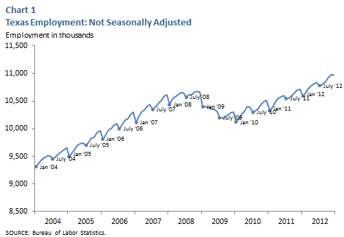
Chart 1 illustrates seasonality in data. The chart plots the raw (that is, not seasonally adjusted) employment data for Texas. (Because it is one of the most widely followed series for the Texas economy, Texas employment data will be used as the example in the remainder of this article.) As the chart shows, the data series exhibits distinctive fluctuating patterns—one obvious pattern being the sharp downward spike each January as temporary holiday hiring comes to a halt. Because of the month-to-month seasonal variations in the data, it is difficult to isolate the actual trend in monthly employment.

Comparing data annually gets around the seasonal problem, but with drawbacks

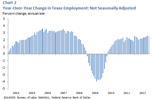
One way analysts avoid the problem of seasonal fluctuation is to compare monthly or quarterly data on a year-over-year basis. In other words, the current month's data point is compared with the data point from the same month in the prior year. A growth rate (or percentage change) is then calculated to get a comparative measure for how fast employment rose or fell over the 12-month period. As shown in Chart 2, this method reduces the fluctuations and can help reveal a trend in the data. However, using the year-over-year method has drawbacks. It relies heavily on data that is 12 months old for the calculations. Comparison from month to month helps economists determine significant changes in the business cycle soon after they occur. Thus, a more sophisticated seasonal adjustment method is called for.

The technical solution

The X13 procedure isolates and removes seasonal factors

Most statisticians, economists and government agencies that report data use a method called the X13 procedure to adjust data for seasonal patterns. The X13 procedure and its predecessor X12, which is still widely used, were developed by the U.S. Census Bureau. [1] When applied to a data series, the X13 process first estimates effects that occur in the same month every year with similar magnitude and direction. These estimates are the “seasonal” components of the data series. In addition, the procedure estimates the “trend-cycle” and “irregular” components. The trend-cycle component is the series' long-term tendency to grow or decline and can fluctuate because of the economic trends or other long-term cyclical factors. The irregular component comes from unseasonable weather, natural disasters, strikes or sampling error. The goal of the seasonal adjustment procedure is to separate out the seasonal component, leaving the trend-cycle and irregular components.

The Census Bureau provides X13 and X12 computer programs free of charge. Additionally, these programs are included in most statistical software. [2]

Many national data series are already seasonally adjusted before they are released. For example, data such as U.S. building permits, housing starts, retail sales, gross domestic product (GDP), the producer price index (PPI) and the consumer price Index (CPI) are released in seasonally adjusted form, simplifying data analysis for economists and business analysts who track the national economy. Some regional data series are not released in seasonally adjusted form, however, and must be adjusted before they can be used in economic analysis.

Real-world example

Seasonally adjusted data show the economic trend

Now let's look at a real-world example to see the effect seasonal adjustment has on a data series. Chart 3 plots both not seasonally Texas employment data and the seasonally adjusted series available from the Dallas Fed. As demonstrated in the chart, the seasonally adjusted series is much smoother and shows a trend in employment. It shows the strong growth in Texas employment from the start of 2014 to early 2020, with a sharp decline with the onset of the COVID-19 pandemic.

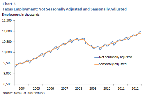
Seasonally adjusted data is especially useful to observe the trend of the data, with the noise of temporary ups and downs removed.

For example, observe the slope of employment growth after 2020. In 2021 and 2022, the slope of job growth was steep as Texas recovered from the pandemic. It would be difficult to tell, looking at the raw data in Chart 1, if 2023 similarly had accelerated growth. But, looking at the seasonally adjusted data in Chart 3, we can see that the slope begins to flatten, suggesting that the rapid growth after mid-2020 started to ease.

Summary

Many types of data exhibit distinct seasonal patterns, which may make it difficult to identify the underlying trend in important economic indicators or make reliable conclusions regarding the current state of the economy. Hence, analysts use the X12 or X13 procedure to separate out seasonal components. This seasonal adjustment process smooths the data series and makes it easier to pinpoint where the economy is heading.

Notes

1. The X13 procedure is an improved version of the X12 method. Enhancements include a more versatile user interface and new tools that help overcome modeling problems, thereby enlarging the range of economic data series that can be adequately seasonally adjusted.
2. For more information on the X13 or X12 procedure, refer to the statistics software manuals or visit the U.S. Census Bureau.